The normal SPC control limit rules display at the 3-sigma level, both high and low. In this case, a simple threshold test determines if a process is in, or out of control. Once a process is brought under control using the simple 3-sigma level tests, quality engineers often want to increase the sensitivity of the control chart, detecting and correcting problems before the 3-sigma control limits are reached. Other, more complex tests rely on more complicated decision-making criteria. These rules utilize historical data and look for a non-random pattern that can signify that the process is out of control, before reaching the normal ±3 sigma limits. The most popular of these are the Western Electric Rules, also know as the WECO Rules, or WE Runtime Rules. First implemented by the Western Electric Co. in the 1920’s, these quality control guidelines were codified in the 1950’s and form the basis for all of the other rule sets. Different industries across the globe have have developed their own variants on the WECO Rules. Other sets of rules, common enough to have an identifying name, i.e. named rules, are listed below.
WECO Runtime and Supplemental Rules – Western Electric Co. – Western Electric Company (1956), Statistical Quality Control handbook. (1 ed.), Indianapolis, Indiana: Western Electric Co., p. v, OCLC 33858387. Sometimes the Supplemental Rules are referred to as the Montgomery Rules, after the statistical quality control expert Douglas Mongtomery. Introduction to Statistical Quality Control (5 ed.), Hoboken, New Jersey: John Wiley & Sons, ISBN 9780471656319
Nelson Rules – The Nelson rules were first published in the October 1984 issue of the Journal of Quality Technology in an article by Lloyd S Nelson.
AIAG Rules– The (AIAG) Automotive Industry Action Group control rules are published in the their industry group “Statistical Process Control Handbook”.
Juran Rules – Joseph M. Juran was an international expert in quality control and defined these rules in his “Juran’s Quality Handbook”, McGraw-Hill Professional; 6 edition (May 19, 2010), ISBN-10: 0071629734
Hughes Rules – The only sources we could find for the Hughes rules were all second hand. If anyone can direct is to an original source for the Hughes Rules, please send an e-mail to support@quinn-curtis.com.
Duncan Rules – Acheson Johnston Duncan was an international expert in quality control and published his rules in the text book “Quality control and industrial statistics” (fifth edition). Irwin, 1986.
Gitlow Rules – Dr. Howard S. Gitlow is an international expert in Sigma Six, TQM and SPC. His rules are found in his book “Tools and Methods for the Improvement of Quality”, 1989, ISBN-10: 0256056803 .
Westgard Rules – The Westgard rules are based on the work of James Westgard, a leading expert in laboratory quality management . They are considered “Laboratory quality control rules”. You can find more information about the Westgard Rules, and James Westgard at the web site: http://www.westgard.com
The rules sets have many individual rules in common. In particular, the WECO rules and the Nelson rules, have 7 out of 8 rules in common, and only differ in the fourth rule. It would seem that the variation in the rule sets are the result of extensive practical experience in different industries. For example,the WECO and Juran rules were developed in the quality systems of Western Electric,which you can consider a manufacturer of electrical consumer and industrial goods. The AIAG rules were developed for the automotive industry. The Westgard rules were developed for laboratory quality systems.
Basic Rules
The Basic Rules are the default rules for all of the SPC charts. They correspond to the ±3-sigma rules used by almost every industry standard SPC chart implementation.
- One of one point is outside of ±3-sigma control limits
Western Electric (WECO) Rules
In the Western Electric Rules A process is considered out of control if any of the following criteria are met:
1. The most recent point plots outside one of the 3-sigma control limits. If a point lies outside either of these limits, there is only a 0.3% chance that this was caused by the normal process.
2. Two of the three most recent points plot outside and on the same side as one of the 2-sigma control limits. The probability that any point will fall outside the warning limit is only 5%. The chances that two out of three points in a row fall outside the warning limit is only about 1%.
3. Four of the five most recent points plot outside and on the same side as one of the 1-sigma control limits. In normal processing, 68% of points fall within one sigma of the mean, and 32% fall outside it. The probability that 4 of 5 points fall outside of one sigma is only about 3%.
4. Eight out of the last eight points plot on the same side of the center line, or target value. Sometimes you see this as 9 out of 9, or 7 out of 7. There is an equal chance that any given point will fall above or below the mean. The chances that a point falls on the same side of the mean as the one before it is one in two. The odds that the next point will also fall on the same side of the mean is one in four. The probability of getting eight points on the same side of the mean is only around 1%.
These rules apply to both sides of the center line at a time. Therefore, there are eight actual alarm conditions: four for the above center line sigma levels and four for the below center line sigma levels.
There are also additional WE Rules for trending and stratification. These are often referred to as WE Supplemental Rules. Don’t rely on the rule number, often these are listed in a different order.
5. Six points in a row increasing or decreasing. The same logic is used here as for rule 4 above. Sometimes this rule is changed to seven points rising or falling.
6. Fifteen points in a row within one sigma. In normal operation, 68% of points will fall within one sigma of the mean. The probability that 15 points in a row will do so, is less than 1%.
7. Fourteen points in a row alternating direction. The chances that the second point is always higher than (or always lower than) the preceding point, for all seven pairs is only about 1%.
8. Eight points in a row outside one sigma. Since 68% of points lie within one sigma of the mean, the probability that eight points in a row fall outside of the one-sigma line is less than 1%.
The rules are described as they appear in the literature. In many cases, a given rule actually specifies two test conditions; the first being a value N out of M above a plus sigma control limit, and the second being a value N out of M below a minus sigma control limit. Examples of this are rules #1, #2 and #3 for WECO and Nelson rules. In other cases, similar rules only contain one test case; N out of M above (or below) a given sigma control limit. Example of this are the Juran rules #2..#5, Hughes Rules #2..#9, Gitlow Rules #2..#5, and Duncan Rules #2..#5.
Nelson Rules
The Nelson rules are almost identical to the combination of the WECO Runtime and Supplemental Rules. It’s not clear why it gets its own name. The only difference is in Rule #4, which changes from 8 out of 8 on one side of the center line to 9 out of 9.
4. Nine out of the last nine points plot on the same side of the center line, or target value.
Statistically, 8 out of 8 test used in the Western Electric Rules has a \((\frac{1}{2})^8\) = 1:256 probability of occurring by chance, while the 9 out of 9 test in the Nelson Rules has a probability of 1:512. Since the standard 3-sigma rules have a probability of 1:370 of occurring by chance, it seems that the Nelson rules decrease the probability of a false alarm as the result of rule #4, below that of rule #1.
AIAG Rules
- One of one point is outside of ±3-sigma control limits
- Seven out of seven are above or below center line
- Seven points in a row increasing
- Seven points in a row decreasing
Juran Rules
- One of one point is outside of ±3-sigma control limits
- Two of three points above 2-sigma control limits
- Two of three points below -2-sigma control limits
- Four of five points is above 1-sigma control limits
- Four of five points is below -1-sigma control limit s
- Six points in a row increasing
- Six points in a row decreasing
- Nine out of nine are above or below center line
- Eight points in a row on both sides of center line, none in zone C
Hughes Rules
- One of one point is outside of ±3-sigma control limits
- Two of three points above 2-sigma control limits
- Two of three points below -2-sigma control limit s
- Three of seven points above 2-sigma control limits
- Three of seven points below -2-sigma control limit s
- Four of ten points above 2-sigma control limits
- Four of ten points below -2-sigma control limits
- Four of five points is above 1-sigma control limits
- Four of five points is below -1-sigma control limits
- Seven points in a row increasing
- Seven points in a row decreasing
- Ten of eleven are above center line
- Ten of eleven are below center line
- Twelve of fourteen are above center line
- Twelve of fourteen are below center line
Gitlow Rules
- One of one point is outside of ±3-sigma control limits
- Two of three points above 2-sigma control limits
- Two of three points below -2-sigma control limits
- Four of five points is above 1-sigma control limits
- Four of five points is below -1-sigma control limits
- Eight points in a row increasing
- Eight points in a row decreasing
- Eight out of Eight are above center line
- Eight out of Eight are below center line
Duncan Rules
- One of one point is outside of ±3-sigma control limits
- Two of three points above 2-sigma control limits
- Two of three points below -2-sigma control limits
- Four of five points is above 1-sigma control limits
- Four of five points is below -1-sigma control limits
- Seven points in a row increasing
- Seven points in a row decreasing
Westgard Rules
- One of one point is outside of ±3-sigma control limits – 13s
- Two of two points outside ±2-sigma control limits – 22s
- Four of four points outside ±-sigma control limits – 41s
- Ten of ten points on one side of center line – 10x
- Two adjacent points on opposite sides of ±-sigma – R4s
- Seven of seven points in a trend increasing or decreasing – 7T
- One of one point is outside of ±-sigma control limits – 12s
- Two of three points outside ±-sigma control limits – 2of32s
- Three of three points outside ±-sigma control limits – 31s
- Six of six points on one side of center line – 6x
- Eight of eight points on one side of center line – 8x
- Nine of nine points on one side of center line – 9x
- Twelve of twelve points on one side of center line – 12x
By default, only the first six Westgard rules described above are enabled. The others can be turned on using the UseNamedRuleSet method and setting ruleflags array elements true for the additional rules. Make sure you use our rule numbers and not the rule numbering above.
The Levey-Jennings chart uses its own subset of these rules:
- One of one point is outside of ±3-sigma control limits – 13s
- Two of two points outside ±2-sigma control limits – 22s
- Four of four points outside ±1-sigma control limits – 41s
- Ten of ten points on one side of center line – 10x
- Two adjacent points on opposite sides of ±2-sigma – R4s
- One of one point is outside of ±2-sigma control limits – 12s
with the others being optional.
- Seven of seven points in a trend increasing or decreasing – 7T
- Two of three points outside ±2-sigma control limits – 2of32s
- Three of three points outside ±1-sigma control limits – 31s
- Six of six points on one side of center line – 6x
- Eight of eight points on one side of center line – 8x
- Nine of nine points on one side of center line – 9x
- Twelve of twelve points on one side of center line – 12x
You can experiment with different rule sets using the interactive app below. It is a bit more complicated than the other ones found on this site, which are mostly specific to one particular SPC chart type.
Named Control Rules – 2 (Interactive)
In the pull-down sections below you find descriptions of the web app setup options. There are six options, divided into three groups you can select from the navigation bar. Click on any of the items below to see a full description.
Setup
Chart Type - Specify the SPC chart type, and sample size for your application.Chart Type
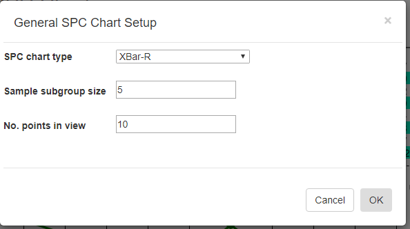
SPC chart type [XBar-R] – select any of the standard SPC chart types: XBar-R, XBar-Sigma, I-R, p-chart, np-chart, c-chart or u-chart.
Sample subgroup size [5]- set the sample subgroup size. If you change the sample subgroup size from the default you should clear the data and simulate new data so that the data uses the new sample subgroup size
Number of points in view[10] – sets the number of sample intervals displayed at a time in the charts and table.
Limits
Control Limits - Specify if control limits are manual or auto-calculated using simple or any of the named control rulesControl Limits
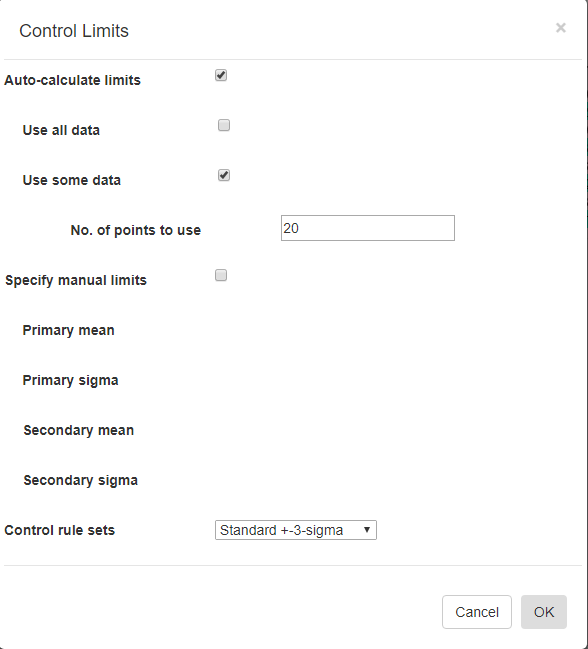
Auto-Calculate limits [Off/On] – Every SPC chart type has a unique way of calculating control limits. Turn this switch On if you want the software to calculate the control limits based on your current data. This option is mutually exclusive with the Specify manual control limits option below.
Use all data [Off/On] – You can use all of the data in the current dataset to calculated the control limits to apply to the dataset. This option is mutually exclusive with the Use some data option below.
Use some data [Off/On] – You can limit the data used in the Auto-Calculate control limits calculation. For example, you can calculate the control limits using the first 20 sample intervals of your dataset, and apply the limits to the remaining intervals of your dataset. This option is mutually exclusive with the Use all data option above.
Nº of points to use [20 ] – Specify the number of sample intervals, starting from the beginning of the current dataset, to use in calculating the control limits
Specify manual limits [Off/On] –You may already know your control limits, because of previously collected data for your process. In that case you can enter the control limit values directly. This option is mutually exclusive with the Auto-Calculate control limits option above.
Primary mean (or target value) [31 ] – Enter the mean value, for the Primary chart. –
Primary 3-Sigma [37.8 ] – Enter the value of the +3 Sigma control limit for the Primary chart. Make sure you enter the +3 Sigma control limit value, and not the +3 Sigma value itself. The +3 Sigma control limit value is the Primary mean (or target) value plus the +3 Sigma value.
Secondary mean (or target value) [11.5 ] – Enter the mean value, (or target value) for the Secondary chart.
Secondary 3-Sigma [4.1 ] – Enter the value of the +3 Sigma control limit for the Secondary chart. Make sure you enter the +3 Sigma control limit value, and not the +3 Sigma value itself. The +3 Sigma control limit value is the Secondary mean (or target) value plus the +3 Sigma value. Also, do not use the +3 Sigma value from the Primary chart. The Secondary chart is going to have its own, unique +3 Sigma value.
Control rule sets [Standard ±3-Sigma] – Regardless of how the control limits are set, automatic or manual, you can specify how those control limits are applied to the underlying data in order to determine whether or not an alarm condition is met. There are nine options: Standard ±3 Sigma, WECO Rules, WECO + SUPP Rules, AIAG Rules, Juran Rules, Hughes Rules, Gitlow Rules, Duncan Rules , Westgard Rules.
Data
Data Simulator -The Data Simulator will generate multiple sample records using just a mean and standard deviation value.Data Simulator
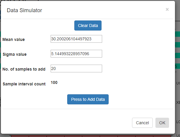
Using the data simulator you can create a randomized dataset for simulated process using just a few parameters. Since the simulated sample data needs to match the [Sample subgroup size] property entered in the SPC Chart Type Setup option, it uses that value when simulating the data.
Difference between Variable and Attribute control charts
The data simulator will automatically take into account whether your SPC chart type is a Variable control chart, or an Attribute control chart. If the chart is a Variable control chart, then N floating point sample values are simulated per sample interval, where N is the sample subgroup size. If the chart is an Attribute control chart, then 1 defect value is simulated for each sample interval, regardless of the sample subgroup size.
[Clear all data] – If you want to start with a empty dataset, select the Clear all data button.
Mean value [30 ] – Enter the mean value you want for the measurement variable. The simulator creates a sample subgroup with randomized values approximating the mean. If you are displaying an Attribute control chart, pick a mean value for defects which reflects what your sample size is. For example, if the subgroup sample size is 100, you should probably have a mean defect rate of at least five to produce reasonable simulated results.
Sigma value [5 ] – Enter the sigma value you want for the measurement variable. This is the approximate sigma value (also known in statistical science as the standard deviation) of the process you want to simulate. Do not confuse this with a sigma control limit. The resulting +3 Sigma control limit is going to be approximately the [Mean value] + 3 * [Sigma value]. Similarly, the -3 Sigma control limit is going to be approximately the [Mean value] – 3 * [Sigma value].
Nº of samples to add [20 ] – Each time you press the [PRESS to add data] button, the specified number of sample intervals will be added to the current dataset. It does NOT automatically clear the dataset. Instead, what you can do is add one batch of N=20 intervals of data using one set of Mean and Sigma values, (30, 2) for example, then you can change the Mean and Sigma slightly, (32, 4) for example, and append another N=20 intervals to the first batch. When setting up the automatic control limits, you can have the software calculate the control limits based on the N =20 samples in the first batch, and watch how those limits detect the process going out of control in the N=20 samples of the second batch.
Sample interval count 50 – Non-editable. Tells you what the current sample interval count is. Each time you press the Add data button, this counter will increment by the value of the Nº of samples to add property above.
[PRESS to add data] – Each time the button is pressed, a batch of simulated sample data is added to the chart dataset. If you want to start over, select the [Clear all data] button.
Recalculate Limits
Force a recalculation of the SPC chart control limits. If one of the Named Rulesets is used that used 1-, 2- and 3-sigma limits, all of the limits are recalculated.
Import Data - You can copy and paste data from an Excel-style spreadsheet into the charts database
Import Data
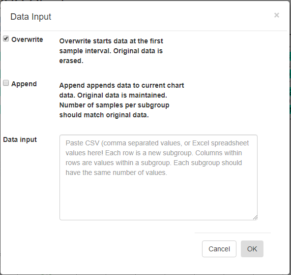
[Overwrite] – Overwrite any current data, starting with the first sample interval.
[Append] – Append data to the current charts data. Original data is maintained. The number of samples per subgroup should match the existing data.
Data input – Paste CSV (comma separated values), or Excel spreadsheet values into this box. Columns within rows are values within a subgroup. Each subgroup should have the same number of values.
If you want to try and plot your own data, you should be able to do so using the Import Data option. Organize your data in a spreadsheet, where the rows represent sample intervals and the columns represent samples within a subgroup. Make sure you only highlight the actual data values, not row or column headings, as in the example below.
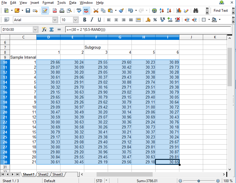
Copy the rectangle of data values from the spreadsheet and Paste them into the Data input box. By default, data values copied from a spreadsheet should be column delimited with the TAB character, and row delimited with the NEWLINE character. If so, our Data input box should be able to parse the data for chart use.
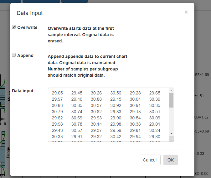
Select OK, and if the data parses properly you should see the resulting data in the chart. By default, data entered into the Data input box overwrites all of the existing data. That way you can create your own custom XBar-R chart, using only your own data. You start by entering in a batch of data
from an “in control” run of your process, and display the data in a new chart. Calculate new control limits based on this data, using the Recalculate Limits button. Should you want to enter in another batch of actual data from a recent run, and append it to the original data, go back to the Import Data menu option. This time select the Append checkbox instead of the default Overwrite data checkbox.