Performance and Process Capability
In SPC, a manufacturing process is often subject to statistical analysis to calculate a simple measure of the overall process capability and performance. The Process Capability measure is generally referred to as Cpk with variants called Cp, Cpl, Cpu and Cpm. The Process Capability (Cpk) measure is meant to be used on a process that is considered to be in statistical control. The Process Performance measures (Ppk, Ppl, Ppu, and Ppk) are meant to be used on a process which is in startup, or is still seeking statistical control.
The process measurement indices are indirectly related to the Variable and Attribute SPC charts discussed elsewhere. They use many of the same intermediate calculations (\(\bar{X}, \bar{R}, \bar{\sigma}\)) as the SPC charts. But the goal of the calculation is different than the Variable and Attribute control charts. The SPC control charts are designed to warn if something is trending wrong with the process, in order that the operator can correct it before you start producing defective parts. The process measurement indices are numerical values which measure how the process is doing compared to preset specification limits.
If you add specification limits to your SPC control charts you will end up with something that looks like the chart below.

Note that the plotted sample values, and the resulting control limits, plot inside the USL=39 and LSL=21 upper and lower specification limits. This should be the case if you are analyzing a process which is both in-control, and capable of producing product within specification limits. Intuitively, the goal is to minimize the variation of the plotted data within the specification limits, subject to economic constraints. At some point the cost to further minimize the product variation is going exceed any expected benefit associated with reducing the variation. So, as long as you are producing within the specification limits, you will reach some level of equilibrium. Important Note – Unlike the SPC control chart 3-sigma limits, which can be calculated automatically if you chose, all of the process measurement indices require that you supply Upper Spec Limit (USL) and Lower Spec Limit (LSL) values. You must set those in the Control Limit setup option, otherwise the results are meaningless.
Rather than just eyeballing it, the process measurement indices calculate a numeric value based on the available data. That way you have some consistent procedure for comparing one production one to another. There are several measurement indices to choose from, so you will need to experiment to use the one most applicable to your particular process.
SPC Process Measurement Nomenclature
USL = Upper Specification Limit
LSL = Lower Specification Limit
\( \tau\) = Tau – Midpoint between USL and LSL = \( \frac{ (LSL + USL)}{2}\)
\( \bar{\bar{X}}\) = XDoubleBar – Mean of sample subgroup means (also called the grand average)
\( \bar{R} \) = RBar – Mean of sample subgroup ranges
\(\sigma \) = Sigma – sample standard deviation – all samples from all subgroups are used to calculate the standard deviation \(\sigma \) .
\( \bar{\sigma} \) = SigmaBar – Average of sample subgroup sigma’s. Each sample subgroup has a calculated standard deviation and the \( \bar{\sigma}\) value is the mean of those subgroup standard deviations. \(d_2\) = a constant tabulated in the section for the XBar-R chart. It is tabulated in any book which discusses the formulation of SPC charts..By convention, the quantity \(\frac{\bar{R}}{d_2}\) is used to estimate the process sigma for the Cp, Cpl and Cpu calculations
Min – a function that returns the lesser of two arguments
Process Capability Ratios (Cp, Cpl, Cpu, Cpk and Cpm)
\( \Large{ Cp =\frac{(USL – LSL)}{ (6 * \frac{\bar{R}}{d_2})}}\)
\( \Large{ Cpu =\frac{(USL -\bar{\bar{X}} )} {(3 * \frac{\bar{R}}{d_2})}}\)
\( \Large{ Cpl = \frac{(\bar{\bar{X}} – LSL)}{(3 * \frac{\bar{R}}{d_2})}} \)
where
\( \Large{V =\frac{\bar{\bar{X}} – \tau}{\sigma}}\)Process Performance Indices (Pp, Ppl, Ppu, Ppk)
\( \Large{ Pp =\frac{(USL – LSL)}{6 * \sigma}}\) \( \Large{ Ppu = \frac{(USL – \bar{\bar{X}} )}{ (3 *\sigma)}}\) \( \Large{ Ppl = \frac{(\bar{\bar{X}} – LSL)}{ (3 * \sigma)}}\) \( \Large{ Ppk = Min(Ppl, Ppu)}\)The major difference between the Process Capability Ratios (Cp, Cpl, Cpu, Cpk) and the Process Performance Indices (Pp, Ppl, Ppu, Ppk) is the estimate used for the process sigma. The Process Capability Ratios use the estimate (\(\frac{\bar{R}}{d_2}\)) and the Process Performance Indices uses the sample standard deviation \(\sigma\). If the process is in control, then Cp vs Pp and Cpk vs Ppk should return approximately the same values, since both (\(\frac{\bar{R}}{d_2}\)) and the sample sigma \(\sigma\) will be good estimates of the overall process sigma. If the process is NOT in control, then ANSI (American National Standards Institute) recommends that the Process Performance Indices (Pp, Ppl, Ppu, Ppk) be used.
Cp and Pp
These measures do not take into account where the process mean is relative to the specification. They merely look at the ratio of spread of the sample interval means with respect to the spread defined by the upper and lower specification limits. So, in one case the process mean can be perfectly centered with respect to the specification limits, while in another case mean can be way off. But the Cp index for both processes can be the same, as long as the standard deviation of the two processes are similar. But, the process which is centered between the specification limits is the one operating most efficiently.
Cpk and Ppk
The Cpk and Ppk measures are an attempt to resolve the Cp and Pp centering issue. They look at the regions above and below the center line separately, and then return the minimum value between the two. This will capture any drift of the process away from the center line, because if the mean value drifts, it will increase the calculated variance in one or the other of the two above or below center line regions . This is done using the intermediate Cpu and Cpl (or Ppu and Ppl) calculations, which are one-sided with respect to the center line. Only the minimum value is returned, so this should better capture if the process is drifting from the mean, or if the overall process variance is increasing compared to the specification limits. The major issue with these calculations is that the process mean and process variation interact in the calculation. So if the process mean is drifting upwards ( reducing the the numerator in the Cpu formula), and the process variance is decreasing (the denominator in the Cpu formula), the two can offset one another and result in the same Cpk values as a perfectly centered process.
Cpm
Cpm is another measure designed to resolve the Cp centering issue. Rather than relying on a minimum operation to choose between Cpu and Cpl, the Cpm calculation incorporates a measure of the degree the process mean is drifting from the target value. If the process is centered on the target, then Cpk and Cpm values for the two processes will be the same. If the process mean drifts from the target, then the Cpm will be lower than the Cpk value.
You can use the interactive program below to experiment with performance measures running on different sets of data and specification limits. See the menu option Performance Measures to set specification limits and select which performance measures you want displayed.
In the pull-down sections below you find descriptions of the web app setup options. There are seven options, divided into three groups you can select from the navigation bar. Click on any of the items below to see a full description.
Setup
Chart Type - Specify the SPC chart type, and sample size for your application.Chart Type
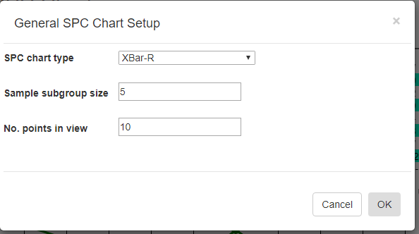
SPC chart type [XBar-R] – select any of the standard SPC chart types: XBar-R, XBar-Sigma, I-R, p-chart, np-chart, c-chart or u-chart.
Sample subgroup size [5]- set the sample subgroup size. If you change the sample subgroup size from the default you should clear the data and simulate new data so that the data uses the new sample subgroup size
Number of points in view[10] – sets the number of sample intervals displayed at a time in the charts and table.
Limits
Control Limits - Specify control limits, either manual or auto-calculated.Control Limits
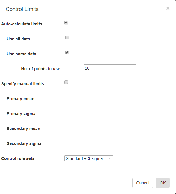
Auto-Calculate limits [Off/On] – Every SPC chart type has a unique way of calculating control limits. Turn this switch On if you want the software to calculate the control limits based on your current data. This option is mutually exclusive with the Specify manual control limits option below.
Use all data [Off/On] – You can use all of the data in the current dataset to calculated the control limits to apply to the dataset. This option is mutually exclusive with the Use some data option below.
Use some data [Off/On] – You can limit the data used in the Auto-Calculate control limits calculation. For example, you can calculate the control limits using the first 20 sample intervals of your dataset, and apply the limits to the remaining intervals of your dataset. This option is mutually exclusive with the Use all data option above.
Nº of points to use [20 ] – Specify the number of sample intervals, starting from the beginning of the current dataset, to use in calculating the control limits
Specify manual limits [Off/On] –You may already know your control limits, because of previously collected data for your process. In that case you can enter the control limit values directly. This option is mutually exclusive with the Auto-Calculate control limits option above.
Primary mean (or target value) [31 ] – Enter the mean value, for the Primary chart. –
Primary 3-Sigma [37.8 ] – Enter the value of the +3 Sigma control limit for the Primary chart. Make sure you enter the +3 Sigma control limit value, and not the +3 Sigma value itself. The +3 Sigma control limit value is the Primary mean (or target) value plus the +3 Sigma value.
Secondary mean (or target value) [11.5 ] – Enter the mean value, (or target value) for the Secondary chart.
Secondary 3-Sigma [4.1 ] – Enter the value of the +3 Sigma control limit for the Secondary chart. Make sure you enter the +3 Sigma control limit value, and not the +3 Sigma value itself. The +3 Sigma control limit value is the Secondary mean (or target) value plus the +3 Sigma value. Also, do not use the +3 Sigma value from the Primary chart. The Secondary chart is going to have its own, unique +3 Sigma value.
Control rule sets [Standard ±3-Sigma] – Regardless of how the control limits are set, automatic or manual, you can specify how those control limits are applied to the underlying data in order to determine whether or not an alarm condition is met. There are nine options: Standard ±3 Sigma, WECO Rules, WECO + SUPP Rules, AIAG Rules, Juran Rules, Hughes Rules, Gitlow Rules, Duncan Rules , Westgard Rules.
Performance Measures
In SPC, a manufacturing process is often subject to statistical analysis to calculate a simple measure of the overall process capability and performance. The most common process measures are Cpk (a Process Capability measure) and Ppk (a Process Performance measure). The Cpk measure is generally preferred when the process is known to be in control, while the Ppk is best used if the process is not in control. Other performance measurement indices include Process Capability indices (Cp, Cpu, Cpl and Cpm) and Process Performance indices (Pp, Ppu, and Ppl).
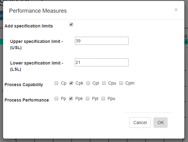
Add specification limits – Specification limits are not the same as sigma-based control limits. The sigma-based control limits are a result of the normal variances of the machines used in the manufacturing process. Specification limits are the tolerance allowed in the finished product to decide whether or not the product meets its targeted quality goals and end-user acceptance. Normally, specification limits for a product in a Six Sigma controlled manufacturing process are going to outside of the ±3 sigma limits. Because who wants a manufacturing process which is incapable of consistently producing a product which meets the quality goals, as specified by the specification limits.
Upper Specification Limit (USL) [40]- Upper Specification limit
Lower Specification Limit (LSL) [20] – Lower Specification limit
Process Capability – Cp, Cpk, Cpl, Cpu, Cpm
Check the process capability indices you want added to the graph.
Process Performance – Pp, Ppk, Ppl, Ppu
Check the process performance indices you want added to the graph.
Data
Data Simulator -The Data Simulator will generate multiple sample records using just a mean and standard deviation value.Data Simulator
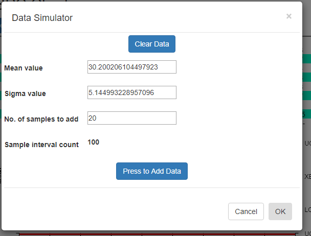
Using the data simulator you can create a randomized dataset for simulated process using just a few parameters. Since the simulated sample data needs to match the [Sample subgroup size] property entered in the SPC Chart Type Setup option, it uses that value when simulating the data.
Difference between Variable and Attribute control charts
The data simulator will automatically take into account whether your SPC chart type is a Variable control chart, or an Attribute control chart. If the chart is a Variable control chart, then N floating point sample values are simulated per sample interval, where N is the sample subgroup size. If the chart is an Attribute control chart, then 1 defect value is simulated for each sample interval, regardless of the sample subgroup size.
[Clear all data] – If you want to start with a empty dataset, select the Clear all data button.
Mean value [30 ] – Enter the mean value you want for the measurement variable. The simulator creates a sample subgroup with randomized values approximating the mean. If you are displaying an Attribute control chart, pick a mean value for defects which reflects what your sample size is. For example, if the subgroup sample size is 100, you should probably have a mean defect rate of at least five to produce reasonable simulated results.
Sigma value [5 ] – Enter the sigma value you want for the measurement variable. This is the approximate sigma value (also known in statistical science as the standard deviation) of the process you want to simulate. Do not confuse this with a sigma control limit. The resulting +3 Sigma control limit is going to be approximately the [Mean value] + 3 * [Sigma value]. Similarly, the -3 Sigma control limit is going to be approximately the [Mean value] – 3 * [Sigma value].
Nº of samples to add [20 ] – Each time you press the [PRESS to add data] button, the specified number of sample intervals will be added to the current dataset. It does NOT automatically clear the dataset. Instead, what you can do is add one batch of N=20 intervals of data using one set of Mean and Sigma values, (30, 2) for example, then you can change the Mean and Sigma slightly, (32, 4) for example, and append another N=20 intervals to the first batch. When setting up the automatic control limits, you can have the software calculate the control limits based on the N =20 samples in the first batch, and watch how those limits detect the process going out of control in the N=20 samples of the second batch.
Sample interval count 50 – Non-editable. Tells you what the current sample interval count is. Each time you press the Add data button, this counter will increment by the value of the Nº of samples to add property above.
[PRESS to add data] – Each time the button is pressed, a batch of simulated sample data is added to the chart dataset. If you want to start over, select the [Clear all data] button.
Recalculate Limits
Force a recalculation of the SPC chart control limits. If one of the Named Rulesets is used that used 1-, 2- and 3-sigma limits, all of the limits are recalculated.
Import Data - You can copy and paste data from an Excel-style spreadsheet into the charts database
Import Data
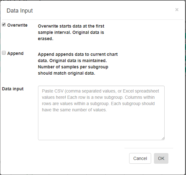
[Overwrite] – Overwrite any current data, starting with the first sample interval.
[Append] – Append data to the current charts data. Original data is maintained. The number of samples per subgroup should match the existing data.
Data input – Paste CSV (comma separated values), or Excel spreadsheet values into this box. Columns within rows are values within a subgroup. Each subgroup should have the same number of values.
If you want to try and plot your own data, you should be able to do so using the Import Data option. Organize your data in a spreadsheet, where the rows represent sample intervals and the columns represent samples within a subgroup. Make sure you only highlight the actual data values, not row or column headings, as in the example below.
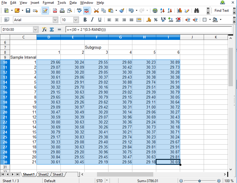
Copy the rectangle of data values from the spreadsheet and Paste them into the Data input box. By default, data values copied from a spreadsheet should be column delimited with the TAB character, and row delimited with the NEWLINE character. If so, our Data input box should be able to parse the data for chart use.
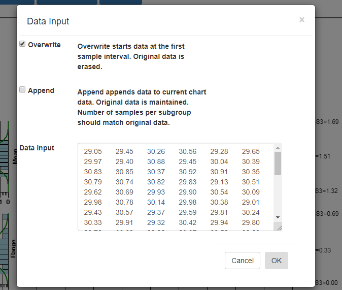
Select OK, and if the data parses properly you should see the resulting data in the chart. By default, data entered into the Data input box overwrites all of the existing data. That way you can create your own custom XBar-R chart, using only your own data. You start by entering in a batch of data
from an “in control” run of your process, and display the data in a new chart. Calculate new control limits based on this data, using the Recalculate Limits button. Should you want to enter in another batch of actual data from a recent run, and append it to the original data, go back to the Import Data menu option. This time select the Append checkbox instead of the default Overwrite data checkbox.